

Repeating a noisy measurement and averaging can make the result more stable. But a larger sample size doesn't correct a biased instrument, nor does it ensure the distribution is well-behaved. This distinction separates the count of observations in a single average from the number of times the experiment is repeated.
What you will be able to explain
Why does having four times as many independent observations reduce the standard deviation of their mean by half? Explain the difference between observations and repeated sample means. Give an example of a distribution where the standard finite-variance argument does not apply.
This experiment uses dimensionless values. Read first: arithmetic averages, square roots, and the idea of a probability distribution. No prior statistics course is required. A physical measurement would include its own units, and its standard deviation would share those units.
Predict
A sensor has independent, identically distributed errors with standard deviation 2 units. If you take the average of 16 readings instead of 4, how does the standard deviation of the average change? Predict the outcome before conducting the experiment. You can skip the question and come back later; nothing is locked.
Manipulate and observe
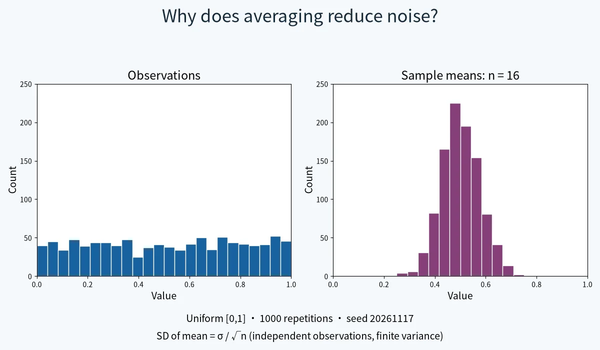
Start with a uniform distribution on [0, 1]. Fix the seed and compare n = 1, 4, 16, and 64. In each trial, n new observations are drawn and one average is recorded. The left histogram shows the first observation from each trial; the right shows the averages. Both use the same horizontal scale. Notice which histogram becomes narrower.
The number of repetitions affects how clearly a histogram shows a distribution. Repetitions are not the observations used in one average. Increasing repetitions from 200 to 1000 results in a cleaner image. It doesn’t alter the theoretical spread of a mean with a fixed sample size.
Try the exponential distribution. The distribution of individual observations is right-skewed. Averages may look different from individual observations. Choose Cauchy last. This is a counterexample, not another instance of the same finite-variance rule. The charts show how many values are outside the displayed range; those values are still included in the numerical summaries.
Explain
For observations that are independent, share the same mean μ, and have finite variance σ², the mean of n observations has an expected value of μ and a variance of σ²/n. Its standard deviation, commonly referred to as the standard error, is σ divided by the square root of n. Increasing the sample size from 4 to 16 reduces the spread by half, not by a factor of four. The expected central value remains unchanged.
Independence is important. When you add variables, their covariance contributes to the variance of the sum. Duplicating a recorded reading does not create independent data. A common offset remains after averaging. That's why multiple sensor readings, biological replicates, and repeated financial data need more than just a large number of samples—the sampling model must match the question.
The central limit theorem deals with the distribution of the standardized sample mean under certain conditions, such as independent and identically distributed observations and a finite, nonzero variance. It doesn't claim that the original data becomes normal. It also doesn't state that any sample size will result in a normal distribution or that a finite simulation confirms the theorem.
The standard Cauchy distribution lacks a population mean and has no finite variance. Thus, the σ/√n formula isn't applicable. In an ideal model, averaging independent standard Cauchy variables results in another standard Cauchy variable. A finite simulation uses pseudorandom numbers with finite precision: it shows heavy tails but can't replicate an infinite tail or prove a limit theorem.
Practice and transfer
Use the two practice questions within the experiment. The first question is about the standard error at a new sample size. The second question asks if averaging eliminates an offset present in all measurements. All feedback remains in this browser tab; the experiment does not store or transmit answers or learning analytics.
Imagine measuring a constant voltage with independent zero-mean random noise and a fixed calibration offset. Which error component shrinks when you average more readings? Why does this distinction still matter when several people share the same instrument? A simulation shows consequences of its assumptions; it cannot determine whether real errors are independent.
Assumptions and reproducibility
Each repetition uses a fresh block of 64 pseudorandom values. The first n numbers are used to calculate the average. Using the same seed and changing n doesn't alter the nested samples. This allows for comparisons between different sample sizes, but the results aren't independent across varying n. Within a single n, each repetition uses a different block of numbers.
The generator uses a 32-bit seed set by the user and is called Mulberry32. Controls are limited: n can be 1, 4, 16, or 64, with a maximum of 3000 repetitions. Uniform, fair Bernoulli, and unit-scale exponential distributions have known means and variances. The Cauchy distribution has neither a mean nor a standard deviation. Empirical standard deviations summarize this finite simulation; they do not establish population moments. Resetting the system restores the default model, seed, and 200 repetitions.
Related ideas
Sampling links mathematics to measurement, computing, and control. Look at the existing PWM and space-vector modulation path for another example of maintaining consistent definitions and measurement values. Check the Math topic page for geometric experiments; these are alternative methods to examine a model, not something required for this lesson.
References
Penn State STAT 414, Mean and Variance of Sample Mean: https://online.stat.psu.edu/stat414/book/export/html/780
StatLect, Central Limit Theorem: https://www.statlect.com/asymptotic-theory/central-limit-theorem
NIST/SEMATECH, Exponential Distribution: https://www.itl.nist.gov/div898/handbook/eda/section3/eda3667.htm
NIST/SEMATECH, Cauchy Distribution: https://www.itl.nist.gov/div898/handbook/eda/section3/eda3663.htm
Concept connections
- Sampling models
- A description of how observations are generated. In this experiment the chosen distribution, independence, and sample size define that model.
- Measurement noise
- Separate random variation from a shared calibration offset before deciding whether repeated readings help.
Continue exploring measurement and control examples. These links extend the idea; they are not prerequisites.